On this page:

Spatial Analysis

Spatial Analysis

Esri Land Cover

Download the zip file and extract the contents to your project folder.

Download datasets

Extracting features by attribute

Open a blank project document.
Add the landuse layer.
Right-click the layer and select Properties.
Click the Information tab in the properties dialog window.
Check and confirm that the CRS is WGS84. You can also check a layer’s CRS by right-clicking on it and selecting Layer CRS.
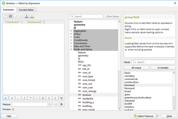
Open the attribute table and click on the Select features using an expression tool to open it.
In the resulting dialog, expand the Fields and Values item in the middle pane, double-click landuse to add to the expression box (left pane).
With landuse still selected, click on All Unique under the Values pane on the right.
In that pane, double-click farmland to add to the expression box. Click Select Features on the lower-right to select the features.

landuse select by expression screenshot

On the title bar of the attribute table, or in the map canvas, you can see the selected features.

On the lower left of the attribute table, click in the box that says Show All Features and select Show Selected Features. How many features are selected?

You will now create a layer of farms from the selected features.

Right-click on the landuse layer and select Export --> Save Selected Features As. Specify the location and file name and save.
Under Format, choose ESRI shapefile and click OK.

Now, in the attribute table, choose to Deselect all features.
Drag and drop the OpenStreetMap under the XYZ Tiles in the Browser panel.
Zoom in to inspect the location of the farms and ascertain if accurate.
Remove the OpenStreetMap layer.

Reprojecting

The current data is in WGS84 Geographic Coordinate System (GCS). Sometimes, you may need to change the CRS of data from different sources into a common CRS. You may also need to add a projected coordinate system to dataset for some spatial analysis. You will change the CRS of the farms dataset. Currently, the project CRS is the same as that of the first layer you added.

Right-click Farms --> Export --> Save Features As. Specify file name and location and choose ESRI shapefile format. In the CRS box, click the Select CRS button.
In the resulting dialog, in the Filter box, type Dominica to search. Choose the Dominica 1945/British West Indies Grid (EPSG: 2002) and press OK.
Press OK again to save the file.

A layer with projected coordinate system (PCS) can be reprojected (transformed) to another PCS. Try transforming the Farms layer with the Dominica 1945 / British West Indies Grid to WGS84 UTM Zone 20N.

In the Processing Toolbox, type project in the search bar.
Double-click Reproject layer.
In the resulting dialog, choose the right layer to be projected as input layer.
For the target CRS, search for UTM and scroll to choose WGS 84 / UTM zone 20N and click Run. The reprojected layer would be added to the map canvas.

Extract Centroids

When you map farms as polygons, you may not need to map them as points. You can extract the central point of the farm. Try this.

In the search bar of the Processing Toolbox, type centroid. * Choose Centroids under the Vector Geometry.
Specify Farms as the input layer. Click on the small arrow in the box to the right of the Centroids box and choose Save to file. Specify the file name and save the layer as a shapefile.
Click Run in the Centroids dialog box. The extracted centroids layer is added.
Zoom in and pan around to explore the centroids. Open the attribute table and note that the centroids layer inherited the attributes of the farms layer.

Calculate Area and Perimeter

Once farms are mapped as polygons, you can calculate the area or perimeter of the farm.

Go to Project --> Properties --> General tab.
Under Measurements, choose meters for units for distance measurement and acres for units for area measurement.
Leave the Display coordinates in map units.
Ensure that the project projection is in WGS 84 / UTM Zone 20N.
Click Apply and OK.

Open the attribute table of the farm layer with the UTM Zone 20N projection.
Click on the Open field calculator button on the attribute table toolbar and choose to Create a new field.
Name the field Area; output field type = decimal number (real); precision = 2.
To calculate the field, expand the Geometry item in the Show Values box.
Double-click $area to add to the expression box and click OK. The calculated area should be added to the table (last column).

In the attribute table, toggle the editing mode off and Save edits.

Remember the unit is same as you specified in the project properties (acres).

Repeat the process in the farm layer with the Dominica 1945 / British West Indies Grid projection.

Compare the area for the farm with ogc_fid 142. Are they the same?

Querying attributes

Make a definition (attribute) query in any of the layers to identify farms with area less than or equal to 2 acres; and those larger than or equal to 10 acres.

Generate statistics

To generate simple statistics for the field Area:

In the Processing Toolbox search bar, search for stat. Choose Basic statistics for fields under the Vector analysis section.
Choose the farm layer as the input layer, and Area as the Field to calculate statistics on. We will keep this as a temporary file so click Run. Once completed, the stats info is displayed under the log tab.

Update farm records with tabular join

Let’s work with the layer having the UTM Zone 20N projection (so remove the other farm layers, if any).

Open the attribute table of this layer and use the Field Calculator to insert a Field with name FarmID.
Expand the variable item and double-click row-number to add to the expression box. Click OK. Row numbers are assigned as IDs under the field FarmID.

We will use this ID to join a hypothetical tabular information collected from the farms.

In the Browser pane, browse to your data folder, drag and drop the FarmAttributes.csv file to the map canvas (it is added to the layers panel).
Right-click the Farms --> Properties --> Joins.
In the resulting dialog, complete the required fields as shown in the figure below.

Joins

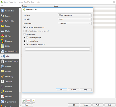
Click OK and OK again to complete the join.
Open the attribute table of the Farms layer and ensure that the fields are joined. The join is temporary, so a new shapefile can be created to make it permanent.
Right-click on the Farms layer --> Export --> Save Features As… save it as shapefile and specify file name and location.
Remove the FarmAttributes.csv file.

Estimate yield (kg/acre)

In the new layer with the join fields, you have average yield of the main crops. Multiplying this by the area should give you an estimated yield.

Open the attribute table of the newly created layer --> Field Calculator. Give a suitable name to the new field, choose decimal number (real) with precision = 2.
Expand the Fields and Values item and make the expression: Area * AvgYield.
Click Ok.
Stop edits and save edits.

The estimated yield of each main crop for each farm is provided in the last column.

Make a definition query to select female farmers who grow dasheen. Your query should look like this: "Sex" = 'F' AND "MainCrop" = 'dasheen'. The query result can also be used to answer the question which female farmer has the largest/smallest area of dasheen.

Generate group statistics

Search again for stat in the Processing Toolbox and choose statistics by category.
In the resulting dialog, choose the newly created join layer as input layer; choose the estimated yield as the field to calculate statistics on (this should be numeric).
Click on the dots next to the box for Field(s) with categories and tick maincrop and sex. Click Run. The output would be seen in the Layers panel as a table. Right-click on it --> Open Attribute Table and view the result, which shows estimated yield statistics by sex and main crop. The count field is the same as frequency. * To save the temporary group statistics layer, right-click and choose make permanent (or export).
Save your project.

Fix geometry and count points in polygon

Some polygon datasets have geometry errors that might only show up during geoprocessing such as overlay. Here, we want to count the number of farms in a given soil class or attributes. We will use the Farm centroids layer. Add the lsd_soil shapefile. Familiarize yourself with the attribute table. In the Processing Toolbox, search for point and choose Count points in polygon under the Vector analysis item.

Complete the dialog box as follows: Polygon = lsd_soil layer; Points = Farmcentroid; Count field name = default.
Click Run.

You may get an error message that the soil layer has geometry errors. You can check which polygons have geometry errors (normally holes in the layer) by using Check validity (under vector geometry) – search for valid in the Processing Toolbox.

In the check validity dialog, choose the soil layer as input and check Ignore ring self intersections.
Click Run to keep all outputs as temporary.

Check the valid and invalid outputs visually.

Repeat the process without checking the Ignore ring self intersections. Are the outputs similar?

Let’s fix the geometry error.

In the Processing Toolbox, find Fix geometries: Input layer = lsd_soil; Repair method = structure; Fixed geometries (choose to save the file with appropriate name).
Click Run.

Now use the soil layer with fixed geometry and run again the Count points in polygon algorithm.
If successful, open the Count layer attribute table. Note that this operation keeps the attributes of the soil layer and adds a field with the count of soil points.
Make an expression to select NUMPOINTS > 0.
Export the selected features to a new shapefile and choose to add the project.
Open the attribute table and explore it.

You will change the field name of NUMPOINTS to something more meaningful.

Edit Field Name

Search for Rename in the Processing Toolbox and choose Rename field.
In the resulting dialog box, choose your Count layer, choose NUMPOINTS for the Field to rename, and give the new name in the New field name box (e.g., NumFarms).

How many farms are in the soil type Kandoid latosol or Young soil (check the Field called type).

Polygon-Polygon Overlay

On the menu bar, go to Vector > Geoprocessing tools > Intersection. Input layer = soil layer with fixed geometries; Overlay layer = Farms layer with the attribute joined. Note: In the Input fields to keep, you can choose which fields in the attribute table of the input layer you want to preserve in the resulting overlay layer. Similarly, in the Overlay fields to keep box, you can choose the fields in the overlay layer to be kept in the resulting layer. Leave these as default for now.
Click Run.

In the resulting layer, examine the attributes. When you do a polygon-polygon overlay, it is always a good idea to re-calculate the geometric area of each polygon feature and not to rely on the previous area.

Use the Field Calculator to calculate the area in a new field and compare the values with the old area in the attribute table.
Now, run Statistics by categories, using the newly calculated area as the Field to calculate statistics on. You can choose the field type as the Field(s) with categories.
Click Run.

Explore the result. Which two soil types are commonest under the farms in the study area? Which soil covers the largest area of farmlands?

Close the table.
Re-run the Statistics by category again, this time add MainCrop and type to the Field(s) with categories box.

Note that this output is temporary (you may make it permanent by saving it if you want). Explore the result. Which crop has the largest area coverage (and on which soil type does it occur)? Ensure that the answer is dasheen on Young soils (if you are not sure, sort the field called sum).

Geometric selection

So far, you have practiced attribute-based selection. Now you will select features based on their geometric or geographic relationship with features in another layer.

Add the lsd_Rivers layer and ppd_Parish layer.

You will subset the Parish layer and use the subset to clip an area of interest from the Rivers layer. Open the attribute table of the Parish layer and select the southern parishes that overlaps with the farms.

Write an expression that looks like in the image below.

select by expression screenshot

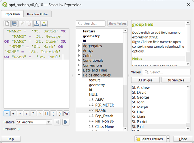
Once the appropriate parishes are selected, export the selected parishes to a new shapefile and choose to add it to the project.
Remove the original parish layer.

Because the Rivers layer is large (covers the whole country), you will clip it to the study parish layer.

On the menu bar, go to Vector > Geoprocessing tools > Clip.
Choose the Rivers layer as input; the subset parish layer as the overlay layer and click Run (if you get error, fix the geometry first and run the clip algorithm again).
Once successful, remove the original Rivers layer. Make the result permanent and save your project.

Select by location

ppd_rivers dataset

On the menu bar, go to Vector > Research Tools > Select By Location. Complete the following: Select Features from: Farms with the attribute joined (the polygon layer), Where the features: intersect, By comparing to the features from: the clipped Rivers layer.
Click Run.
Open the attribute table of farms layer and choose to show selected features. How many farms intersect rivers?
In the map canvas, turn off all the layers except the farms layer, zoom in to see which farms were selected.

Select within a distance

You will now select features based on distance to features in another layer. Example, you might be interested in which farms are within a given distance of a protected area.

In the Processing Toolbox, expand the Vector Selection --> Select within distance. Select Features From: Farmcentroids; By comparing to the features from: clipped Rivers layer; Where the features are within: 50 meters
Click Run.
Open the Farmcentroids attribute table and check how many features are selected to be within 50 meters of rivers.

Extract raster values to points

You might be interested in the elevation of a given farm location. You can extract the elevation from a digital elevation model (DEM) using point features.

Add the Voidfilled_DEM raster data and then the Farmcentroids layer.

Note that the DEM layer is unprojected and has WGS84 GCS.

In the Processing Toolbox, go to Raster Analysis --> Sample raster values. Input layer: Farmcentroids; Raster layer: Voidfilled_DEM; Output column prefix = ELEV_
Click Run.
Open the Farmcentroids attribute table and check the last column or field to see the extracted elevation values for the farm locations. You may use the Identify tool to explore the elevations of a few farms.

Zonal Statistics

Add the Void_filled DEM raster data. You can reproject (warp) to WGS84 / UTM Zone 20N.
Add the Parish layer you used previously to the map.
In the Processing toolbox, search for ‘zonal’ and choose Zonal statistics.
- Input layer: parishes;
- Raster layer: DEM;
- Output column prefix: ELEV_
- Statistics to calculate: click the 3 dots and choose Mean, Minimum, Maximum
You may choose to save the Zonal statistics output layer.
Click Run.
Open the attribute table of the resulting zonal statistics output layer and look for the statistics calculated (in the last columns, with the prefix ELEV_).

Zonal Histogram

For each Dominica parish, you will calculate zonal histogram to summarize the pixel count of each land cover/use class in the ESRI land cover/use layers for the 2018 and 2022.

First, clip the land cover/use layer with the coastline layer.

In the Processing toolbox, search for ‘clip’ and choose Clip raster by mask layer under the GDAL (Raster extraction) function.
Input layer = land use/cover raster. Mask layer = coastline. Ensure that the Match the extent of the clipped raster to the extent of the mask layer is checked.
Click Run.
Make the output or result permanent by exporting it as a Geotiff.
After saving the clipped layers, remove the temporary clipped layers and the original land use/cover layers. You may as well remove the coastline layer.
Colour the clipped layers by assigning the land use/cover classes obtainable from the Class Definitions table below.
Double-click one of the clipped layers to open the property window.
Click the Symbology tab.
- Render type = Paletted/Unique values;
- Click Classify at the bottom left to see the classes and labels.
- Under label, double click on a class number and type in the right name obtained from the metadata. The class numbers are below:

Class definitions table

Class (Value)	Name	Description
1	Water	Areas where water was predominantly present throughout the year; may not cover areas with sporadic or ephemeral water; contains little to no sparse vegetation, no rock outcrop nor built up features like docks; examples: rivers, ponds, lakes, oceans, flooded salt plains.
2	Trees	Any significant clustering of tall (~15 feet or higher) dense vegetation, typically with a closed or dense canopy; examples: wooded vegetation, clusters of dense tall vegetation within savannas, plantations, swamp or mangroves (dense/tall vegetation with ephemeral water or canopy too thick to detect water underneath).
4	Flooded vegetation	Areas of any type of vegetation with obvious intermixing of water throughout a majority of the year; seasonally flooded area that is a mix of grass/shrub/trees/bare ground; examples: flooded mangroves, emergent vegetation, rice paddies and other heavily irrigated and inundated agriculture.
5	Crops	Human planted/plotted cereals, grasses, and crops not at tree height; examples: corn, wheat, soy, fallow plots of structured land.
7	Built area	Human made structures; major road and rail networks; large homogenous impervious surfaces including parking structures, office buildings and residential housing; examples: houses, dense villages / towns / cities, paved roads, asphalt.
8	Bare ground	Areas of rock or soil with very sparse to no vegetation for the entire year; large areas of sand and deserts with no to little vegetation; examples: exposed rock or soil, desert and sand dunes, dry salt flats/pans, dried lake beds, mines.
9	Snow/ice	Large homogenous areas of permanent snow or ice, typically only in mountain areas or highest latitudes; examples: glaciers, permanent snowpack, snow fields.
10	Clouds	No land cover information due to persistent cloud cover.
11	Rangeland	Open areas covered in homogenous grasses with little to no taller vegetation; wild cereals and grasses with no obvious human plotting (i.e., not a plotted field); examples: natural meadows and fields with sparse to no tree cover, open savanna with few to no trees, parks/golf courses/lawns, pastures. Mix of small clusters of plants or single plants dispersed on a landscape that shows exposed soil or rock; scrub-filled clearings within dense forests that are clearly not taller than trees; examples: moderate to sparse cover of bushes, shrubs and tufts of grass, savannas with very sparse grasses, trees or other plants.

Credit: Sentinel-2 10m Land Use/Land Cover Time Series

Change colours of the layers: Once the class labels are assigned, you can double-click individual colours beside the labels and change them to suit your preference.

Try changing the colour of one class, click Apply to see how it looks like on the map. Complete the styling of the map.
You can save the style to use in the future. At the lower left of the property dialog, click Style --> Save Style and browse to save it at a desired location.
To use the saved style on a different layer, open the property dialog of the layer to be styled, click Style --> Load style and browse to the saved style.

Alternatively, you can click OK in the current property dialog to exit. You can then copy the style:

Right-click the stylized layer –> Copy style.
Then, right-click the other layer –> Paste style. Explore the maps for accuracy based on your local knowledge.
Add the parishes layer. In the Processing toolbox, search for ‘zonal histogram’.
- Raster layer = one of the land use/cover layers.
- Vector layer containing zones = Parishes.
- Leave the rest as default.
Click Run.
Open the output table of the result, look for the columns with HISTO_ as the suffix to see the number of pixels (or pixel count) for each land use/cover class in each parish.
Calculate area of crop:
- Check the pixel size of the land use/cover layer under the information tab in the properties dialog. Note that it is 10 m. Confirm this information with the metadata of the land use/cover layer.
  - Go to Project --> Properties --> General tab. Ensure that the units for area measurement is in meters. Close the project property dialog.

The land use/cover class 5 denotes crops. Let’s calculate the area of crops in each parish.

Click on the Field Calculator on the toolbar of the attribute table.
Ensure that the Create a new field is checked.
Name the new field CropArea
- Datatype = Decimal number
- Field length = 10
- Precision = 2
- In the expression box, multiply the HISTO_5 field by 10 by 10 (the cell area of the land use/cover layer as seen from the metadata). Your expression should look like:
  
  “HISTO_5” * 10 * 10
Click OK to evaluate the expression.
Check the result in the attribute table (note that the area is in square meters).

Explore the results.

Which parish has the largest/smallest crop area?
Compute area of trees and indicate which parishes have the largest/smallest area of trees.

You can also map the parishes based on any of the attributes (e.g. crop area or number of trees).

Raster Calculator: you can use the raster Calculator to apply mathematical functions to one or more raster layers. Here, you will multiply the 2022 layer by 10 or 100.

In the Processing toolbox, search for calculator and choose Raster calculator.
In the dialog box, double-click on the 2022 raster layer to add it to the expression box.
Click * to add to the box and type 10 (or 100, whichever you prefer) into the box.
Scroll down to set the cell size or the layer from which cell size and CRS should be obtained.
Click Run.

Examine the output to note the cell values have changed but the data (map) itself is not changed. This is simply a reclassification.